Can you Prove it... combinatorially?

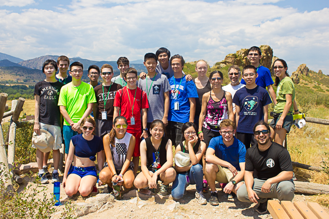
This year’s Prove it! Math Academy was a big success, and it was an enormous pleasure to teach the seventeen talented high school students that attended this year. Some of the students mentioned that they felt even more inspired to study math further after our two-week program, but the inspiration went both ways - they inspired me with new ideas as well!

One of the many, many things we investigated at the camp was the Fibonacci sequence, formed by starting with the two numbers $0$ and $1$ and then at each step, adding the previous two numbers to form the next: \[0,1,1,2,3,5,8,13,21,\ldots\] If $F_n$ denotes the $(n+1)$st term of this sequence (where $F_0=0$ and $F_1=1$), then there is a remarkable formula for the $n$th term, known as Binet’s Formula:

\[F_n=\frac{1}{\sqrt{5}}\left( \left(\frac{1+\sqrt{5}}{2}\right)^n - \left(\frac{1-\sqrt{5}}{2}\right)^n \right)\]

Looks crazy, right? Why would there be $\sqrt 5$’s showing up in a sequence of integers?

PhinisheD!

Sometimes it’s the missteps in life that lead to the greatest adventures down the road.

For me, my pursuit of a Ph.D. in mathematics, specifically in algebraic combinatorics, might be traced back to my freshman year as an undergraduate at MIT. Coming off of a series of successes in high school math competitions and other science-related endeavors (thanks to my loving and very mathematical family!), I was a confident and excited 18-year old whose dream was to become a physicist and use my mathematical skills to, I don’t know, come up with a unified field theory or something.

But I loved pure math too, and a number of my friends were signed up for the undergraduate Algebraic Combinatorics class in the spring, so my young ambitious self added it to my already packed course load. I had no idea what “Algebraic Combinatorics” even meant, but I did hear that it was being taught by Richard Stanley, a world expert in the area. How could I pass up that chance? What if he didn’t teach it again before I left MIT?

What do Schubert curves, Young tableaux, and K-theory have in common? (Part III)

This is the third and final post in our expository series of posts (see Part I and Part II) on the recent paper coauthored by Jake Levinson and myself.

Last time, we discussed the fact that the operator $\omega$ on certain Young tableaux is actually the monodromy operator of a certain covering map from the real locus of the Schubert curve $S$ to $\mathbb{RP}^1$. Now, we’ll show how our improved algorithm for computing $\omega$ can be used to approach some natural questions about the geometry of the curve $S$. For instance, how many (complex) connected components does $S$ have? What is its genus? Is $S$ a smooth (complex) curve?

What do Schubert curves, Young tableaux, and K-theory have in common? (Part II)

In the last post, we discussed an operation $\newcommand{\box}{\square} \omega$ on skew Littlewood-Richardson Young tableaux with one marked inner corner, defined as a commutator of rectification and shuffling. As a continuation, we’ll now discuss where this operator arises in geometry.

Schubert curves: Relaxing a Restriction

Recall from our post on Schubert calculus that we can use Schubert varieties to answer the question:

Given four lines $\ell_1,\ell_2,\ell_3,\ell_4\in \mathbb{C}\mathbb{P}^3$, how many lines intersect all four of these lines in a point?

What do Schubert curves, Young tableaux, and K-theory have in common? (Part I)

In a recent and fantastic collaboration between Jake Levinson and myself, we discovered new links between several different geometric and combinatorial constructions. We’ve weaved them together into a beautiful mathematical story, a story filled with drama and intrigue.

So let’s start in the middle.

Slider puzzles for mathematicians

Those of you who played with little puzzle toys growing up may remember the “15 puzzle”, a $4\times 4$ grid of squares with 15 physical squares and one square missing. A move consisted of sliding a square into the empty square. The French name for this game is “jeu de taquin”, which translates to “the teasing game”.