
What is a $q$-analog? (Part 1)
Hi, I’m Maria and I’m a $q$-analog addict. The theory of $q$-analogs is a little-known gem, and in this series of posts I’ll explain why they’re so awesome and addictive!
So what is a $q$-analog? It is one of those rare mathematical terms whose definition doesn’t really capture what it is about, but let’s start with the definition anyway:
Definition: A $q$-analog of a statement or expression $P$ is a statement or expression $P_q$, depending on $q$, such that setting $q=1$ in $P_q$ results in $P$.
So, for instance, $2q+3q^2$ is a $q$-analog of $5$, because if we plug in $q=1$ we get $5$.
Glencoe/McGraw-Hill doesn't believe this bijection exists
Education is a difficult task, it really is. Teaching takes a few tries to get the hang of. Writing textbooks is even harder. And math is one of those technical fields in which human error is hard to avoid. So usually, when I see a mistake in a math text, it doesn’t bother me much.
But some things just hurt my soul.

No correspondence between the integers and rationals? Yes there is, Example 2! Yes there is!
The r-major index
In this post and this one too, we discussed the inv and maj statistics on words, and two different proofs of their equidistribution. In fact, there is an even more unifying picture behind these statistics: they are simply two different instances of an entire parameterized family of statistics, called $r\text{-maj}$, all of which are equidistributed!
Deriving the discriminant of a cubic polynomial through analytic geometric means
This is a contributed gemstone, written by Sushant Vijayan. Enjoy!
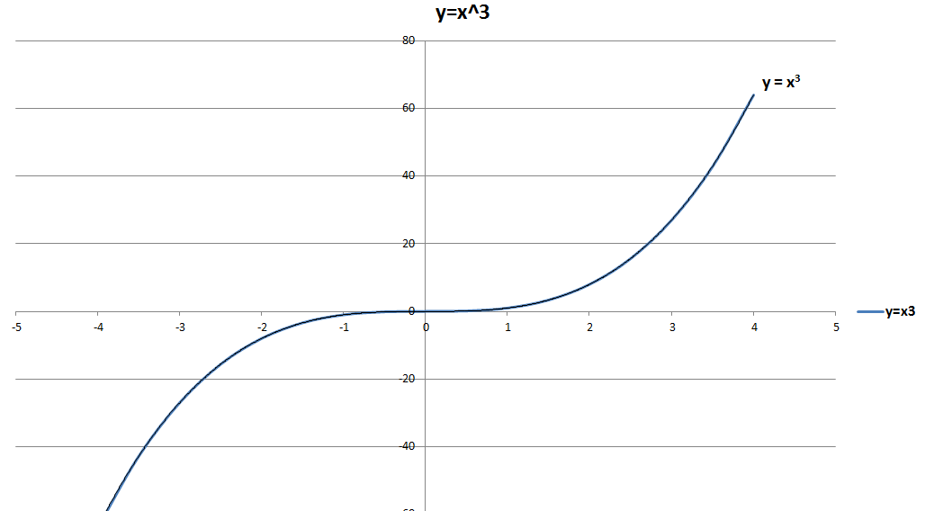
Consider a generic cubic equation \[at^3+bt^2+ct+d=0,\] where $a,b,c,d$ are real numbers and $a \neq 0$. Now we can transform this equation into a depressed cubic equation, i.e., one with no $t^2$ term, through means of Tschirnhaus Transformation $t=x-\frac{b}{3a}$, followed by dividing through by $a$. The depressed cubic equation is given by \[x^3+px+q=0\] where $p$ and $q$ are related to $a,b,c,d$ by the relation given here. Setting $p=-m$ and $q=-n$ and rearranging we arrive at \[x^3 =mx+n \hspace{3cm} (1)\] We will investigate the nature of roots for this equation. We begin with plotting out the graph of $y=x^3$:
The Springer Correspondence, Part III: Hall-Littlewood Polynomials
This is the third post in a series on the Springer correspondence. See Part I and Part II for background.
In this post, we’ll restrict ourselves to the type A setting, in which $\DeclareMathOperator{\GL}{GL}\DeclareMathOperator{\inv}{inv} G=\GL_n(\mathbb{C})$, the Borel $B$ is the subgroup of invertible upper triangular matrices, and $U\subset G$ is the unipotent subvariety. In this setting, the flag variety is isomorphic to $G/B$ or $\mathcal{B}$ where $\mathcal{B}$ is the set of all subgroups conjugate to $B$.
The Hall-Littlewood polynomials
For a given partition $\mu$, the Springer fiber $\mathcal{B}_\mu$ can be thought of as the set of all flags $F$ which are fixed by left multiplication by a unipotent element $u$ of Jordan type $\mu$. In other words, it is the set of complete flags \[F:0=F_0\subset F_1 \subset F_2 \subset \cdots \subset F_n=\mathbb{C}^n\] where $\dim F_i=i$ and $uF_i=F_i$ for all $i$.