The Garsia-Procesi Modules: Part 2

This is a long overdue followup post to Garsia-Procesi Modules: Part 1 that I finally got around to editing and posting. Enjoy!

In this post, I talked about the combinatorial structure of the Garsia-Procesi modules $R_\mu$, the cohomology rings of the type A Springer fibers. Time to dive even further into the combinatorics!

Tanisaki generators, visually

Recall that, for a partition $\mu$ of $n$, the graded $S_n$-module $R_\mu$ can be constructed (due to Tanisaki) as the quotient ring \[\mathbb{C}[x_1,\ldots,x_n]/I_\mu\] where $I_\mu$ is generated by certain partial elementary symmetric functions called Tanisaki generators.

Define $d_k(\mu)=\mu’_{n-k+1}+\mu’_{n-k+2}+\cdots$ to be the sum of the last $k$ columns of $\mu$, where we pad the conjugate partition $\mu’$ with $0$’s in order to think of it as as a partition of $n$ having $n$ parts. Then the partial elementary symmetric function $e_r(x_{i_1},\ldots,x_{i_k})$ is a Tanisaki generator if and only if $k-d_k(\mu)\lt r\le k$. Tanisaki and Garsia and Procesi both use this notation, but I find $d_k$ hard to remember and compute with, especially since it involves adding zeroes to $\mu$ and adding parts of its transpose in reverse order, and then keeping track of an inequality involving it to compute the generators.

An equivalent, and perhaps simpler, definition is as follows. If $n-k\lt \mu_1$, then the quantity $k-d_k(\mu)$ is equal to the number of squares in the first $n-k$ columns of $\mu$, excluding the first row. Indeed, we have \[k-d_k(\mu)=n-d_k(\mu)-(n-k),\] and on the right hand side, $n-d_k(\mu)$ is simply the number of squares in the first $n-k$ columns of $\mu$. Subtracting $n-k$ is then equivalent to removing one square from each column in that count, which can be done by crossing out the first row of $\mu$.

So, define \[s_t(\mu)=\mu’_1+\cdots+\mu’_t-t\] to be the number of squares in the first $t$ columns, not including the first row. Then we include an elementary symmetric function $e_r$ in $k$ of the variables $x_i$ if \[r\gt s_{n-k}(\mu).\] (Note that the upper bound condition, $r\le k$, is necessary for the elementary symmetric function to be nonzero, so we technically don’t need to state the upper bound).

For instance, if $n=8$ and $\mu=(4,3,1)$, then the partition diagram looks like:

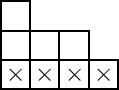
where the bottom row is x’ed out to remind ourselves not to count it.

For $k=8$, we require $r\gt s_0(\mu)=0$, so all elementary symmetric functions $e_1,\ldots,e_8$ in the $8$ variables $x_1,\ldots,x_8$ are in $I_\mu$.

For $k=7$ we require $r\gt s_1(\mu)=2$, so $e_3,e_4,\ldots,e_7$ on any seven of the variables are generators.

For $k=6$ we require $r \gt s_2(\mu)=3$, so $e_4,e_5,e_6$ on any six of the variables are generators.

For $k=5$ we require $r \gt s_3(\mu)=4$, so only $e_5$ on any five of the variables is a generator.

For $k=4$ we require $r\gt s_4(\mu)=4$, and we have no additional generators.

For $k$ such that $n-k>\mu_1$, we also never get any additional generators, since $k-d_k(\mu)=k$ in this case. Therefore the combinatorial interpretation above, which is only valid for $n-k<\mu_1$, is in fact an equivalent definition for the Tanisaki generators.

It’s not fundamentally all that different, but working with columns of a partition from the left rather than the right can save a bit of mental space during computations.

A smaller set of generators, visually

Another way to encode the calculations above is by writing the elementary symmetric functions in the empty boxes above, in order from left to right and up the columns. And note that if $e_r(S)$ is in the ideal for all sets of variables $S$ with $|S|=k$, then $e_r(S’)$ is in the ideal for $|S’| \gt k$ as well, because we can simply take the sum of all $e_r(B)$ for subsets $B\subseteq S$ of size $k$ and we obtain a constant multiple of $e_r(S)$ by symmetry. Thus we do not need to list, for instance, $e_3$ in all $8$ variables when we also already have $e_3$ in all sets of $7$ variables. So, the generators we need are, in this case, shown below:

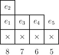
where the numbers below each column indicate how many variables the partial $e_i$’s in that column are considered in. Note that here this gives the generating set

\[(e_1,e_2,e_3(7),e_4(6),e_5(5))\]

where $e_3(7)$ indicates the set of all $e_3(S)$ where $S$ is a subset of the variables of size $7$, and similarly for the other partial elementary symmetric functions.

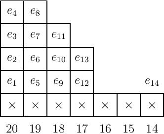
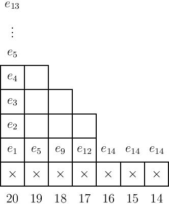
As a larger example, we compute below the ideal $I_\lambda$ for $\lambda=(7,4,4,3,3)$ by writing the elementary symmetric functions in the empty boxes up each column in order from left to right. We then consider the contributions from the columns to the right of all boxes in rows above the first; note that this starts at $e_{14}$ for each of these columns, and so it suffices to only list $e_{14}$ in all subsets of $14$ variables, in other words, only place the $e_{14}$ in the column labeled $14$. This will then generate all other $e_{14+i}(S)$ for $|S|>14$, and so our set of generators is as shown in the diagram.

In general, we will require a single $e_i$ to be written in the final column, whose column label is also $i$, outside of the empty boxes. When the first several rows have equal length, we simply place it on top of the last column, as in the example below:

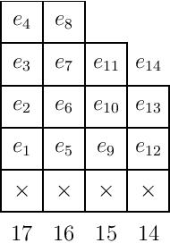
This $e_i$, along with the elementary symmetric functions written in the boxes, gives a full set of generators for $I_\lambda$.

An alternative smaller set of generators

In this section we will show that, for $|S| < n$, it suffices to only include $e_r(S)$ for the smallest possible $r$, along with $e_1,\ldots,e_n$ in all of the variables, in order to generate the Tanisaki ideal. We prove this here.

Visually, this looks like taking only the following generators:

(Note that we could include up to $e_{20}$ in all $20$ variables in the first column, but since we have $e_{14}$ in $14$ variables, all other $e_k$ for $k\ge 14$ vanish as well.)

To see why this is sufficient, we note that, for instance, the “missing” generator $e_{6}(x_1,\ldots,x_{19})$ can be generated as follows: \[e_{6}(x_1,\ldots,x_{19})=e_6(x_1,\ldots,x_{19},x_{20})-x_{20}e_5(x_1,\ldots,x_{19}).\] We can then inductively show from left to right that all of the generators that “fill in” the rest of the tableau are generated as well.

We now write out a full proof of the ideas above. Write $X={x_1,\ldots,x_n}$ throughout.

Proposition. The ideal $I_\mu$ is generated by the following elements:

The elementary symmetric functions $e_1,\ldots,e_n$ in all $n$ variables $x_1,\ldots,x_n$, and
The partial elementary symmetric functions $e_r(S)$ where $S\subseteq X$ with $|S| = k < n$ and \[r=s_{n-k}(\mu)+1.\]

Proof. Let $I_\mu^0$ be the ideal generated by the above functions. To show $I_\mu^0=I_\mu$, it suffices to show that for every $k<n$ and $r\gt s_{n-k}(\mu)$, $e_r(S) \in I_\mu^0$. We show this by nested strong induction, first on $n-k$ and then on $r$.

For the base case, $n-k=0$, we have $k=n$ and all of the elementary symmetric functions on all $n$ variables are in $I_\mu^0$ by its definition. Now fix $k$ and assume the claim holds for all smaller values of $n-k$ (for all larger values of $k$). Let $S\subseteq X$ with $|S| =k$, and since $k<n$, choose a missing variable $x_i\in X-S$.

Define $r_0=s_{n-k}(\mu)+1$; we have $e_{r_0}(S)\in I_\mu^0$ by the definition of $I_\mu^0$. Now let $r>r_0$ and assume $e_t(S)\in I_\mu^0$ for all $t$ such that $r_0\le t\le s_{n-(k+1)}(\mu)$. Then $e_r(S\cup \{x_i\})\in I_\mu^0$ by the induction hypothesis on $n-k$. Therefore \[e_r(S)=e_r(S\cup \{x_i\}) - x_i e_{r-1}(S)\in I_\mu^0\] as desired. QED

Recursive algorithm for expanding in basis $\mathcal{B}(\mu)$

Garsia and Procesi define a basis $\mathcal{B}(\mu)$ of monomials for $R_\mu$ recursively by \[\mathcal{B}(\mu)=\bigcup_i x_n^{i-1}\mathcal{B}(\mu^{(i)}).\] (Recall that $\mu^{(i)}$ is the partition of $n-1$ formed by removing one square from the $i$th part and re-sorting the resulting rows in partition order.) They then give a completely elementary inductive proof that every other element of $R_\mu$ can be expressed as a linear combination of basis elements from $\mathcal{B}(\mu)$. We describe their algorithm here, with a few slight modifications.

First, note that it suffices to describe how to express any monomial $x^\alpha$ as a linear combination of the elements of $\mathcal{B}_\mu$, plus an element of $I_\mu$. For $n=0$, the only partition is the empty partition, $R_\emptyset=\mathbb{C}$, and the unique basis element is $1$, so $x^\alpha=x^0=1$ is its entire expansion (since $I_\emptyset=(0)$).

For $n>0$, we use the following recursive algorithm.

Given $x^\alpha=x_1^{\alpha_1}\cdots x_n^{\alpha_n}$, let $i-1=\alpha_n$ be the exponent of $x_n$.
Setting $\beta=(\alpha_1,\ldots,\alpha_{n-1})$, we have that $x^{\beta}=x_1^{\alpha_1}\cdots x_{n-1}^{\alpha_{n-1}}$ can be interpreted as a representative of an element in $R_{\mu^{(i)}}$. Use this algorithm recursively to express $x^\beta$ in terms of $\mathcal{B}(\mu^{(i)})$ plus an error term in $I_{\mu^{(i)}}$, giving an expansion \[x^\beta=\sum_{b\in \mathcal{B}(\mu^{(i)})} c_b b(x_1,\ldots,x_{n-1}) +E\] where $E\in I_{\mu^{(i)}}$.
Multiplying both sides by $x_n^{i-1}$, we have \[x^\alpha=\sum_{b\in \mathcal{B}(\mu^{(i)})}c_bx_n^{i-1}b(x_1,\ldots,x_{n-1})+x_n^{i-1}E.\] Each monomial $x_n^{i-1}b(x_1,\ldots,x_{n-1})$ is an element of $\mathcal{B}(\mu)$ by the recursive definition of the basis $\mathcal{B}(\mu)$.
We next expand $x_n^{i-1}E$ as a linear combination of elements of $\mathcal{B}(\mu)$ plus an element of $I_\mu$. Since $E\in I_{\mu^{(i)}}$, we can write \[E=\mathop{\sum_{r>s_{n-k}(\mu^{(i)})}}_{i_1,\ldots,i_k\in [n-1]} a_{r,\{i_j\}}e_r(x_{i_1},\ldots,x_{i_k}).\] We will consider each term individually, expressing $x_n^{i-1}e_r(x_{i_1},\ldots,x_{i_k})$ in terms of $I_{\mu}$ plus elements of $x_n^{i}R_\mu$ (hence reducing to a case in which the exponent of $x_n$ is larger, at which point we can repeat the algorithm until the exponent is above $\mu’_1$.)
If either $n-k\lt \mu_i$, or if $n-k\ge \mu_i$ and $r>s_{n-1-k}(\mu^{(i)})+1=s_{n-1-k}(\mu)$, then $e_r(x_{i_1},\ldots,x_{i_k},x_n)\in I_\mu$ and so the expansion \[x_n^{i-1}e_r(x_{i_1},\ldots,x_{i_k})=x_n^{i-1}e_r(
x_{i_1},\ldots,x_{i_k} ,x_n)-x_n^ie_{r-1}(x_{i_1},\ldots,x_{i_k})\] is our desired expression in $I_\mu+x^iR_\mu$.
Otherwise, if $n-k\ge \mu_i$ and $r=s_{n-1-k}(\mu^{(i)})+1=s_{n-1-k}(\mu)$, then note that we must have $i>1$. Iteratively using the identity $x_ne_r(x_{i_1},\ldots,x_{i_k})=e_{r+1}(x_{i_1},\ldots,x_{i_k},x_n)-e_{r+1}(x_{i_1},\ldots,x_{i_k})$, we can multiply by $x_n$ exactly $i-1$ times to obtain \[\begin{align*} x_n^{i-1}e_r(x_{i_1},\ldots,x_{i_k})= & \phantom{+}x_n^{i-2}e_{r+1}(x_{i_1},\ldots,x_{i_k},x_n) \\ &-x_n^{i-3}e_{r+2}(x_{i_1},\ldots,x_{i_k},x_n) \\ &+\cdots \\ &+ (-1)^{i-2}e_{r+i-1}(x_{i_1},\ldots,x_{i_k},x_n) \\ &+(-1)^{i-1}e_{r+i-1}(x_{i_1},\ldots,x_{i_k})\end{align*}\] all of whose terms on the right hand side are in $I_\mu$.
We now have expressed each term of $E$ in the form $I+x_n^iE_1$ where $I\in I_\mu$ is expressed in terms of the Tanisaki generators, and $E_1\in R_\mu$. We iterate steps 1-6 on each term of $x_n^iE_1$ and continue until we only have monomials having $x_n^h$ as a factor where $h=\mu_1’$ is the height of $\mu$.
Note that \[\begin{align*}x_n^h= &\phantom{+}x_n^{h-1}e_1(x_1,\ldots,x_n) \\ &-x_n^{h-2}e_2(x_1,\ldots,x_n) \\ &+\cdots \\ &+(-1)^{h-1}e_h(x_1,\ldots,x_n) \\ &-e_h(x_1,\ldots,x_{n-1}). \end{align*}\] The first $h$ terms above are clearly in $I_\mu$, and the last term $e_h(x_1,\ldots,x_{n-1})$ is in $I_\mu$ as well because $h>s_{n-(n-1)}(\mu)=\mu’_1-1$. The above expansion, as well as the similar relations for $x_i^h$ obtained by acting by an appropriate element of $S_n$, ensures that the process terminates.

We can now use this algorithm to express every monomial of degree at most $n(\mu)=\sum_i (i-1)\mu_i$ (which is the highest nonzero degree of $R_\mu$) in terms of the basis $\mathcal{B}(\mu)$ plus an element of $I_\mu$, expressed explicitly in terms of Tanisaki generators.

In order to minimize recursive calls, one should build this database of expansions starting with partitions of size $1$, then of size $2$, and so on. Further, for a given partition shape $\mu$, one should first expand the monomials of degree at most $n(\mu)$ with the highest possible exponent of $x_n$ (namely $x_n^h$ where $h=\mu_1’$ and then continue with the monomials having $n$th exponent $x_n^{h-1}$, then with $x_n^{h-2}$, and so on. This ensures that steps 4-8 of the algorithm only need to be run once on each summand in the error term $E$ obtained in step 3.

Expansions up to $|\mu|=3$

Using the above algorithm, I was able to quickly calculate all monomial expansions of degree at most $n(\mu)$ for all partitions $\mu$ of size at most $3$ by hand. In some cases, I worked out some of the expansions of the monomials of degree larger than $n(\mu)$, which lie entirely in $I_\mu$, as a convenience for the calculations in the subsequent cases. (In general, if one were to code this algorithm with the goal of finding the expansions for $R_\mu$, one should calculate the $I_{\lambda}$ expansions for all monomials of degree up to $n(\mu)$ for ALL partitions $\lambda\le \mu$, in order to maximize efficiency at each step.)

For $\mu=(1)$, we have $\mathcal{B}((1))=\{1\}$ and $I_\mu=(e_1(x_1))$. The expansions are:

$x_1=e_1(x_1)$
$1=1$

For $\mu=(2)$, we have $\mathcal{B}((1))=\{1\}$ and $I_\mu=(e_1(x_1,x_2),e_2(x_1,x_2),e_1(x_1),e_1(x_2))$. The expansions are:

$x_2=e_1(x_2)$
$x_1=e_1(x_1)$
$1=1$

For $\mu=(1,1)$, we have $\mathcal{B}((1))=\{1,x_2\}$ and $I_\mu=(e_1(x_1,x_2),e_2(x_1,x_2))$. The expansions are:

$x_2^2=x_2e_1(x_1,x_2)-e_2(x_1,x_2)$
$x_2x_1=e_2(x_1,x_2)$
$x_2=x_2$
$x_1^2=x_1e_1(x_1,x_2)-e_2(x_1,x_2)$
$x_1=-x_2+e_1(x_1,x_2)$
$1=1$

For $\mu=(3)$, we have $\mathcal{B}((1))=\{1\}$ and $I_\mu$ is the set of all partial elementary symmetric functions in three variables, so $R_\mu=\mathbb{C}$. The expansions are:

$1=1$

For $\mu=(2,1)$, we have $\mathcal{B}((1))=\{1,x_2,x_3\}$ and $I_\mu=(e_1,e_2,e_3,e_2(x_1,x_2),e_2(x_1,x_3),e_2(x_2,x_3))$, where $e_i$ without any variables indicates the full elementary symmetric functions using all three variables. The expansions are:

$x_3^2=x_3e_1-e_2+e_2(x_1,x_2)$
$x_3=x_3$
$x_2=x_2$
$x_1=-x_3-x_2+e_1$
$1=1$

For $\mu=(1,1,1)$, we have $\mathcal{B}((1))=\{1,x_2,x_3,x_3x_2,x_3^2,x_3^2x_2\}$ and $I_\mu=(e_1(x_1,x_2,x_3),e_2(x_1,x_2,x_3),e_3(x_1,x_2,x_3))$. For shorthand in this case we simply write $e_1,e_2,e_3$ since there are no strictly partial $e_r$’s in $I_\mu$. The expansions are:

$x_3^3=x_3^2e_1-x_3e_2+e_3$
$x_3^2x_2=x_3^2x_2$
$x_3^2x_1=-x_3^2x_2+x_3e_2-e_3$
$x_3^2=x_3^2$
$x_3x_2^2=-x_3^2x_2+(x_2x_3+x_3^2)e_1-x_3e_2$
$x_3x_1^2=x_3^2x_2+(x_3^2+x_3x_1)e_1
-2x_3e_2 +e_3$
$x_3x_2x_1=e_3$
$x_3x_2=x_3x_2$
$x_3x_1=-x_3x_2-x_3^2+x_3e_1$
$x_3=x_3$
$x_2^3=x_2^2e_1-x_2e_2+e_3$
$x_2^2x_1=x_3^2x_2-x_2x_3e_1+x_2e_2$
$x_2^2=-x_3x_2+(x_2+x_3)e_1-e_2$
$x_2x_1^2=-x_3^2x_2-x_1x_3e_1+(x_1+x_3)e_2-e_3$
$x_2x_1=x_3^2-x_3e_1+e_2$
$x_2=x_2$
$x_1^3=x_1^2e_1-x_1e_2+e_3$
$x_1^2=x_3x_2+x_3^2-x_1e_1-e_2$
$x_1=-x_2-x_3+e_1$
$1=1$